Module SampleRepresentation

Deals with the sample representation for simulation of the reflectivity.

A multilayer sample is represented by a Heterostructure object. Its main pupose is to deliver the list of layers (Layer type of the Pythonreflectivity package from Martin Zwiebler) with defined susceptibilities at certain energies via :meth.`Heterostructure.getSingleEnergyStructure`. The layers within this heterostructure are represented by instances of LayerObject or of derived classes, which alows for a very flexibel modelling of the sample.

So far the following layer types are implemented:

• LayerObject: Layer with a constant (over energy) but fittable electric susceptibility tensor.
• ModelChiLayerObject: This layer type holds the electric susceptibility tensor as a user-defined function of energy.
• MagneticLayerObject: This layer type deals with a magnetic layer and therefor creates the off-diagonal elements of the susceptibitlity tensor from a magnetic term and two angles.
• AtomLayerObject: This layer deals with compositions of atoms with different formfactors. The densities of the atoms can be varied during fitting procedures and plotted with using plotAtomDensity(). The formfactors are represented by instances of classes which are derived from Formfactor (the base class is abstract and cannot be used directly).

So far the following formfactor types are implemented:

• FFfromFile: Reads an energy-dependent formfactor as data points from a textfile. For energies between the data points the formfactor is linearly interpolated.
• FFfromScaledAbsorption: Reads an absorption measurement (fitted to off-resonant tabulated values) and a theoretical/tabulated energy-dependen formfactor from textfiles. Within a given energy-range, the absorption is scaled with a fittable factor and the real part is obtained by a Kramers-Kronig transformation. See section 3.3 of Martin Zwiebler PhD-Thesis for details.
• FFfromFitableModel: Formfactor from user-defined fitable model functions. Can be used to implement e.g. a Kramers-Kronig variational approach.
• MagneticFormfactor: Basic formfactor class to deal with a magnetic formfactor, i.e. only the off-diagonal elements of a formfactor tensor. Magnetic terms are defined by the user as instances of Parameters.ParametrizedFunction.
• MFFfromXMCD: A magnetic formfactor which is created from an XMCD measurement.

To allow for atomic slicing you can create density profiles with class DensityProfile or the specialized DensityProfile_erf. Once created, they can provide atomic densities used in AtomLayerObject for the different layers (which are used as slices).

The function plotAtomDensity() can be used to plot the variation of atom densities between the layers.

class SampleRepresentation.Heterostructure(number_of_layers=0, multilayer_structure=None)

Bases: object

Represents a heterostructure as a stack of instances of LayerObject or of derived classes. Its main pupose is to model the sample in a very flexibel way and to get the list of layers (Layer type of the Pythonreflectivity package from Martin Zwiebler) with defined susceptibilities at certain energies.

In contrast to Martin’s list of Layer-type objects, this class contains all information also for different energies.

__init__(number_of_layers=0, multilayer_structure=None)

Create heterostructructure object.

Parameters:

• number_of_layers (int) – gives the number of different layers
• multilayer_structure (list) – Makes it possible to define multilayers which contain identical layers several times. This can be done by passing a list containing the indices of layers from the lowest (e.g. substrate) to the highest (top layer, hit first by the beam). Default is [0,1,2,3, ...,number_of_layers-1]. Multilayer syntax is e.g.``[0,1,2,[100,[3,4,5,6]],7,.,1,..]`` which repeats 100 times the sequence of layers 3,4,5,6 in between 2 and 7 and later on layer 1 is repeated once.

setLayout(number_of_layers, multilayer_structure=None)

Change the layout of the heterostructure.

See __init__() for details. Only difference is: you cannot make changes which would remove layers.

setLayer(index, layer)

Place layer (instance of LayerObject) at position index (counting from 0, starting from the bottom or according to indices defined by multilayer_structure).

getLayer(index)

Return the instance of LayerObject which is placed at position index (counting from 0, starting from the bottom or according to indices defined by multilayer_structure).

getTotalLayer(index)

Return the instance of LayerObject which is placed at position index (counting from 0, starting from the bottom, repeated layers are counted repeatedly).

removeLayer(index)

Remove the instance of LayerObject which is placed at position index (counting from 0, starting from the bottom or according to indices defined by multilayer_structure).

index can also be a list of indices. BEWARE: The instance of LayerObject itself and the corresdonding instances of Parameters.Fitparameter are not deleted! So in a following fitting procedure, these parameters might still be varied even though they don’t have any effect on the result.

getSingleEnergyStructure(fitpararray, energy=None)

Return list of layers (Layer type of the Pythonreflectivity package from Martin Zwiebler) which can be directly used as input for Pythonreflectivity.Reflectivity().

energy in units of eV

N

(int) Number of different layers. Read-only.

N_total

(int) Total number of layers counting also multiple use of the same layer according to multilayer_structure. Read-only.

class SampleRepresentation.LayerObject(chitensor=None, d=None, sigma=None, magdir='0')

Bases: object

Base class for all layer objects as the common interface. Speciallized implementation should inherit from this class.

__init__(chitensor=None, d=None, sigma=None, magdir='0')

Parameters:

• d (Parameters.Parameter) – Thickness. Unit is the same as for every other length used throughout the project and is not predefined. E.g. wavelength. None or 0 mean infinitively thick.
• sigma (Parameters.Parameter) – The roughness of the upper surface of the layer. Has dimension of length. Unit: see d.
• chitensor (list of Parameters.Parameter) –

  Electric susceptibility tensor of the layer.

  • [chi] sets chi_xx = chi_yy = chi_zz = chi
  • [chi_xx,chi_yy,chi_z] sets chi_xx,chi_yy,chi_zz, others are zero
  • [chi_xx,chi_yy,chi_z,chi_g] sets chi_xx,chi_yy,chi_zz and depending on magdir chi_yz=-chi_zy=chi_g (if x), chi_xz=-chi_zx=chi_g (if y) or chi_xz=-chi_zx=chi_g (if z)
  • [chi_xx,chi_xy,chi_xz,chi_yx,chi_yy,chi_yz,chi_zx,chi_zy,chi_zz] sets all the corresdonding elements
• magdir (str) – Gives the magnetization direction for MOKE. Possible values are “x”, “y”, “z” and “0” (no magnetization).

getChi(fitpararray, energy=None)

Return the electric susceptibility tensor as a list of numbers for a certain energy corresponding to the parameter values in fitpararray (see Parameters).

The returned list can be of length 1,3,4 or 9 (see __init__()). For the base implementation of LayerObject the parameter energy is not used. But it may be used by derived classes like AtomLayerObject and therefore needed for compatibility.l energy is measured in units of eV.

getD(fitpararray)

Return the thickness of the layer as a number corresponding to the parameter values in fitpararray (see Parameters).

The thickness is given in the unit of length you chose. You are free to choose whatever unit you want, but use the same for every length troughout the project.

getSigma(fitpararray)

Return the roughness of the upper surface of the layer as a number corresponding to the parameter values in fitpararray (see Parameters).

The thickness is given in the unit of length you chose. You are free to choose whatever unit you want, but use the same for every length troughout the project.

getMagDir(fitpararray=None)

Return magnetization direction

fitpararray is not used and just there to give a common interface. Maybe a derived classes will have a benefit from it.

d

Thickness of the layer. Unit is the same as for every other length used throughout the project and is not predefined. E.g. wavelength.

chitensor

Electric susceptibility tensor of the layer. See __init__() for details.

sigma

Roughness of the upper surface of the layer. Unit is the same as for every other length used throughout the project and is not predefined. E.g. wavelength.

magdir

Magnetization direction for MOKE. Possible values are “x”, “y”, “z” and “0” (no magnetization).

class SampleRepresentation.MagneticLayerObject(chi_diag, m_prime, m_primeprime, theta_M, phi_M, d=None, sigma=None)

Bases: SampleRepresentation.LayerObject

Specialized layer to deal with a magnetic layer without energy-dependence.

The electrical suszeptibility tensor (Chi) consists of an energy-independent diagonal part and of off-diagonal elements which are given as a magnetization and their direction (angles).

__init__(chi_diag, m_prime, m_primeprime, theta_M, phi_M, d=None, sigma=None)

Initializes the MagneticLayerObject with both diagonal-elements and off-diagonal elements given as magnetic terms m_prime and m_primeprime and the angles theta_M and phi_M which describe the direction of the magnetization.

See Macke and Goering 2014, J.Phys.: Condens. Matter 26, 363201. Eq. 11-14 for details.

Parameters:

• chi_diag (list of Parameters.Parameter) –

  Diagonal elements of electric susceptibility tensor of the layer.

  • [chi] sets chi_xx = chi_yy = chi_zz = chi
  • [chi_xx,chi_yy,chi_z] sets chi_xx,chi_yy,chi_zz
• m_prime (Parameters.Parameter) –
• m_primeprime (Parameters.Parameter) – Real and imaginary parts of the magnetic term.
• theta_M (Parameters.Parameter) –
• phi_M (Parameters.Parameter) – Angles which describe the direction of the magnetization measured in degrees. See also Geometry / Coordinate System.
• d (Parameters.Parameter) – Thickness. Unit is the same as for every other length used throughout the project and is not predefined. E.g. wavelength. None or 0 mean infinitively thick.
• sigma (Parameters.Parameter) – The roughness of the upper surface of the layer. Has dimension of length. Unit: see d.

class SampleRepresentation.ModelChiLayerObject(chitensorfunction, d=None, sigma=None, magdir='0')

Bases: SampleRepresentation.LayerObject

Speciallized layer to deal with an electrical suszeptibility tensor (Chi) which is modelled as function of energy.

BEWARE: The inherited property chitensor is now a function.

__init__(chitensorfunction, d=None, sigma=None, magdir='0')

Parameters:

• d (Parameters.Parameter) – Thickness. Unit is the same as for every other length used throughout the project and is not predefined. E.g. wavelength. None or 0 mean infinitively thick.
• sigma (Parameters.Parameter) – The roughness of the upper surface of the layer. Has dimension of length. Unit: see d.
• chitensorfunction (Parameters.ParametrizedFunction) –

  Energy-dependent electric susceptibility tensor of the layer. A parametrized function of energy (see Parameters.ParametrizedFunction) which reurns a list of either 1,3,4 or 9 real or complex numbers. See also documentation of Pythonreflectivity.

  • [chi] sets chi_xx = chi_yy = chi_zz = chi
  • [chi_xx,chi_yy,chi_z] sets chi_xx,chi_yy,chi_zz, others are zero
  • [chi_xx,chi_yy,chi_z,chi_g] sets chi_xx,chi_yy,chi_zz and depending on magdir chi_yz=-chi_zy=chi_g (if x), chi_xz=-chi_zx=chi_g (if y) or chi_xz=-chi_zx=chi_g (if z)
  • [chi_xx,chi_xy,chi_xz,chi_yx,chi_yy,chi_yz,chi_zx,chi_zy,chi_zz] sets all the corresdonding elements
• magdir (str) – Gives the magnetization direction for MOKE. Possible values are “x”, “y”, “z” and “0” (no magnetization).

getChi(fitpararray, energy)

Return the electric susceptibility tensor as a list of numbers for a certain energy corresponding to the parameter values in fitpararray (see Parameters).

energy is measured in units of eV.

chitensor

Electric susceptibility tensor of the layer. Is an instance of Parameters.ParametrizedFunction. See __init__() for details.

class SampleRepresentation.AtomLayerObject(densitydict={}, d=None, sigma=None, magdir='0', densityunitfactor=1.0)

Bases: SampleRepresentation.LayerObject

Speciallized layer class to deal with compositions of atoms and their energy dependent formfactors (which can be obtained from absorption spectra).

Especially usefull to deal with atomic layers, but can also be used for bulk. The atoms and their formfactors have to be registered a the class (with registerAtom) before they can be used to instantiate a new AtomLayerObject. The atom density can be plotted with plotAtomDensity(). Density is measured in mol/cm$^3$ (as long as no densityunitfactor is applied)

Used formfactors can also be “magnetic formfactors” which only deal with diagonal elements of a formfactor tensor and simulate magnetic moments. See MagneticFormfactor and derived classes.

__init__(densitydict={}, d=None, sigma=None, magdir='0', densityunitfactor=1.0)

Parameters:

• densitydict – a dictionary which contains atom names (strings, must agree with before registered atoms) and densities (must be instances of Parameters.Parameter or of a derived class).
• d (Parameters.Parameter) – Thickness. Unit is the same as for every other length used throughout the project and is not predefined. E.g. wavelength. None or 0 mean infinitively thick.
• sigma (Parameters.Parameter) – The roughness of the upper surface of the layer. Has dimension of length. Unit: see d.
• densityunitfactor (float) –

  If the densities in densitydict are measured in another unit than mol/cm^3, state this value which translates your generic density to the one used internally. I.e.:

  rho_in_mol_per_cubiccm = densityunitfactor * rho_in_whateverunityouwant
  

getDensitydict(fitpararray=None)

Return the density dictionary either with evaluated paramters (needs fitpararray) or with the raw Parameters.Parameter objects (use fitparraray = None).

getChi(fitpararray, energy)

Return the electric susceptibility tensor as a list of numbers for a certain energy corresponding to the parameter values in fitpararray (see Parameters).

energy is measured in units of eV.

classmethod registerAtom(name, formfactor=None)

Register an atom called name for later use to instantiate an AtomLayerObject.

formfactor as to be an instance of Formfactor or of a derived class. If no formfactor object is given, an instance of FFfromChantler will be created with name as element name. This can be used for an easy registration of atoms with just their tabulated formfactors from the Chantler tables.

classmethod getAtom(name)

Return the Formfactor object registered for atom name.

classmethod getAtomNames()

Return a list of names of registered atoms.

class SampleRepresentation.Formfactor

Bases: object

Base class to deal with energy-dependent atomic form-factors.

This base class is an abstract class an cannot be used directly. The user should derive from this class if he wants to build his own models.

See Formfactor and Susceptibility for sign conventions.

__init__()

Initialize self. See help(type(self)) for accurate signature.

getFF(energy, fitpararray=None)

Return the formfactor for energy corresponding to fitpararray (if it depends on it) as 9-element Numpy array of complex numbers.

energy is measured in units of eV.

plotFF(fitpararray=None, energies=None)

Plot the energy-dependent formfactor with the energies (in eV) listed in the list/array energies. If this array is not given the plot covers the hole existing energy-range. The fitpararray has only to be given in cases where the formfactor depends on a fitparamter, e.g. for class:FFfromScaledAbsorption.

maxE

Upper limit of stored energy range. Read-only.

minE

Lower limit of stored energy range. Read-only.

class SampleRepresentation.FFfromFile(filename, linereaderfunction=None, energyshift=<sphinx.ext.autodoc.importer._MockObject object>)

Bases: SampleRepresentation.Formfactor

Class to deal with energy-dependent atomic form-factors (entire tensor) which are tabulated in files. See Formfactor and Susceptibility for sign conventions.

__init__(filename, linereaderfunction=None, energyshift=<sphinx.ext.autodoc.importer._MockObject object>)

Initializes the FFfromFile object with an energy-dependent formfactor given as file.

Parameters:

• filename (str) – Path to the text file which contains the formfactor.
• linereaderfunction (callable) – This function is used to convert one line from the text file to data. It should be a function which takes a string and returns a tuple or list of 10 values: (energy,f_xx,f_xy,f_xz,f_yx,f_yy,f_yz,f_zx,f_zy,f_zz), where energy is measured in units of eV and formfactors are complex values in units of e/atom (dimensionless). It can also return None if it detects a comment line. You can use FFfromFile.createLinereader() to get a standard function, which just reads this array as whitespace seperated from the line.
• energyshift (Parameters.Parameter) – Species a fittable energyshift between the energy-dependent formfactor from filename and the real one in the reflectivity measurement. So the formfactor delivered from FFfromFile.getFF() will not be formfactor_from_file(E) but formfactor_from_file(E-energyshift).

static createLinereader(complex_numbers=True)

Return the standard linereader function for usage with FFfromFile.__init__().

This standard linereader function reads energy and complex elements of the formfactor tensor as a whitespace-seperated list (i.e. 10 numbers) and interpretes “#” as comment sign. If complex_numbers = False then the reader reads real and imaginary part of every element seperately, i.e. every line has to consist of 19 numbers seperated by whitespaces:

energy f_xx_real ff_xx_im ... f_zy_real f_zy_im f_zz_real f_zz_im

getFF(energy, fitpararray=None)

Return the (energy-shifted )formfactor for energy as an interpolation between the stored values from file as 9-element 1-D numpy array of complex numbers.

Parameters:

• energy (float) – Measured in units of eV.
• fitpararray – Is actually only needed when an energyshift has been defined.

maxE

Upper limit of stored energy range. Read-only.

minE

Lower limit of stored energy range. Read-only.

class SampleRepresentation.FFfromChantler(element_symbol, energyshift=<sphinx.ext.autodoc.importer._MockObject object>)

Bases: SampleRepresentation.FFfromFile

Class to create an atomic formfactor for an element from Database (Chantler Tables taken from https://dx.doi.org/10.18434/T4HS32).

__init__(element_symbol, energyshift=<sphinx.ext.autodoc.importer._MockObject object>)

Initializes the FFfromChantler object with an energy-dependent formfactor corresponding to the element given with element_symbol.

Parameters:

• element_symbol (str) – Refers to the element of which the atomic formfactor should be looked up. (More specifically: name of the corresponding database file without suffix.)
• energyshift (Parameters.Parameter) – Species a fittable energyshift between the energy-dependent formfactor from Chantler Tables and the real one in the reflectivity measurement. So the formfactor delivered from FFfromChantler.getFF() will not be formfactor_from_database(E) but formfactor_from_databayse(E-energyshift).

class SampleRepresentation.FFfromScaledAbsorption(element_symbol, E1, E2, E3, scaling_factor, absorption_filename, absorption_linereaderfunction=None, energyshift=<sphinx.ext.autodoc.importer._MockObject object>, autofitfunction=None, autofitrange=None, tabulated_filename=None, tabulated_linereaderfunction=None)

Bases: SampleRepresentation.Formfactor

A formfactor class which uses the imaginary part of the formfactor (experimentally determined absorption signal which has been fitted to off-resonant values) given as a file, scales it with a fittable factor and calculates the real part by the Kramers-Kronig transformation. It realizes the procedure described in section 3.3 of Martin Zwiebler PhD-Thesis. It thereby deals only with the diagonal elements of the formfactor tensor. For the off-diagonal elements, the magnetic formfactors classes are used.

See Formfactor and Susceptibility for sign conventions.

__init__(element_symbol, E1, E2, E3, scaling_factor, absorption_filename, absorption_linereaderfunction=None, energyshift=<sphinx.ext.autodoc.importer._MockObject object>, autofitfunction=None, autofitrange=None, tabulated_filename=None, tabulated_linereaderfunction=None)

Initializes the FFfromScaledAbsorption object with an energy-dependent imaginary part of the formfactor given as file.

To perform the Kramers-Kronig transformation without integrating to infinity, theoretical/tabulated formfactors (Chantler tabels from https://dx.doi.org/10.18434/T4HS32) are used. Their imaginary part differs only close to resonance from the measured absorption and should have been used before to perform the fit of the measured absorption to off-resonant values.

The imaginary part of each element of the formfactor is:

• the value given by Im_f0_E1, for energy < E1.
• the value given by the file scaled by scaling_factor (roughly, see PhD Thesis of Martin Zwiebler,section 3.3, for details), for E1 <= energy <= E2
• linear inperpolation between the scaled value at E2 and the value given for E3 by Im_f0_E3, for E2 < energy < E3
• the value given by Im_f0_E3, for E3 < energy

The Kramers-Kronig transformation to obtain the real part is done only once during instantiation. Therefore, it does not have to be repeated with every value of the scaling_factor and fitting is fast.

Parameters:

• element_symbol (string) – States the chemical element for which this formfactor is created as usual short version of its name. It is important to lookup the tabulated/theoretical reference formfactors from the Chantler tables. If you want to use your own formfactor as reference (see arguments tabulated_filename and tabulated_linereaderfunction) just enter an empty string here.
• E1 (float) – Energy in eV. From this energy on the energy-dependent imaginary part of the formfactor given as file is used and scaled.
• E2 (float) – Energy in eV. From this energy on the imaginary part of the formfactor is linearly interpolated.
• E3 (float) – Energy in eV. From this energy on the imaginary part of the formactor is constant Im_f_E3.
• scaling_factor (Parameter.Parameter) – Specifies the fittable scaling factor (called a in Martin Zwiebler PhD Thesis).
• absorption_filename (str) – Path to the text file which contains the imaginary part of the formfactor which results from an apsorption measurement and a subsequent fit to off-resonant tabulated values.
• absorption_linereaderfunction (callable) – This function is used to convert one line from the absorption text file to data. It should be a function which takes a string and returns a tuple or list of 4 values: (energy, Im f_xx, Im f_yy, Im f_zz), where energy is measured in units of eV and imaginary parts of formfactors are real values in units of e/atom (dimensionless). It can also return None if it detects a comment line. You can use FFfromScaledAbsorption.createAbsorptionLinereader() to get a standard function, which just reads this array as whitespace seperated from the line. This is actually the default if you give ‘None’.
• energyshift (Parameters.Parameter) – Species a fittable energyshift between the energy-dependent formfactor calculated by the whole above mentioned procedure and the real one in the reflectivity measurement. As a consequence the peak but also E1,E2 and E3 are shifted.
• autofitfunction (callable) –
• autofitrange (float) – If given together with autofitfunction, the absorbtion from absorbtion_filename will be fitted to the imaginary part of the formfactors from Chantler tables or tabulated_filename just below/above E1/E3 in a range given by autofitrange in eV. More specifically autofifunction will be fitted to the f2 of the Chantler tables. autofitfunction must work as following f2=func(energy,absorbtion,a,b,c,…). absorbtion is the measured absorbtion/TEY/FY/… at a certain energy and a,*b*,*c*, … are an arbitrary number of parameters. The parameters will be fitted such that the return values fit best to the f2 of the Chantler tables in the given energy-range. E.g. a standard fitfunction would be: f2(E) = absorbtion*energy*a + b + c energy. (see Martin Zwiebler PhD-Thesis, section 3.3)
• tabulated_filename (str) – Path to the text file which contains the tabulated/theoretical formfactor for the corresponding element. You can use this argument if you dont’t want to use the standard Chantler tables. But therefore element_symbol has to be an empty string
• tabulated_linereaderfunction (callable) – This function is used to convert one line from the tabulated text file to data. It should be a function which takes a string and returns a tuple or list of 2 values: (energy,f), where energy is measured in units of eV and the formfactor f is a complex value in units of e/atom (dimensionless). It can also return None if it detects a comment line. You can use FFfromScaledAbsorption.createTabulatedLinereader() to get a standard function, which just reads this array as whitespace separated from the line. This is actually the default if you give ‘None’. You can use this argument if you dont’t want to use the standard Chantler tables and want to create your own linereader.

static createAbsorptionLinereader()

Return the standard linereader function for absorption files for usage with FFfromScaledAbsorption.__init__().

This standard linereader function reads energy and elements of the imaginary part of the formfactor tensor as a whitespace-seperated list (i.e. 4 numbers) and interpretes “#” as comment sign.

static createTabulatedLinereader(complex_numbers=True)

Return the standard linereader function for tabulated formfactor files for usage with FFfromScaledAbsorption.__init__().

This standard linereader function reads energy and the complex formfactor as a whitespace-seperated list (i.e. 2 numbers) and interpretes “#” as comment sign. If complex_numbers = False then the reader reads real and imaginary part of the formfactor seperately, i.e. every line has to consist of 3 numbers seperated by whitespaces:

energy ff_real ff_im

getFF(energy, fitpararray)

Return the (energy-shifted )formfactor for energy as an interpolation between the stored values from file as 9-element 1-D numpy array of complex numbers.

Parameters:

• energy (float) – Measured in units of eV.
• fitpararray – Is needed for the scaling factor ‘a’ and an energy shift if defined.

maxE

Upper limit of stored energy range. Read-only.

minE

Lower limit of stored energy range. Read-only.

class SampleRepresentation.FFfromFitableModel(ff_tensor_function, minE, maxE)

Bases: SampleRepresentation.Formfactor

Formfactor class which can used to implement a fittable model for the formfactor as e.g. a Kramers-Kronig variational approach with triangles (see Stone et al., PRB 86, 024102 (2012).

The class just take the complex formfactor tensor as Parameters.ParametrizedFunction, which is a function dependent on fitparameters.

See Formfactor and Susceptibility for sign conventions.

__init__(ff_tensor_function, minE, maxE)

Parameters:

• ff_tensor_function (Parameters.ParametrizedFunction) – Energy-dependent complex formfactor tensor. A parametrized funtion of energy (see Parameters.ParametrizedFunction) which reurns a list of 9 complex numbers.
• minE (float) –
• maxE (float) – Gives the boundaries of the valid energy-range of the given ff_tensor_function.

getFF(energy, fitpararray=None)

Return the formfactor for energy corresponding to fitpararray (if it depends on it) as 9-element Numpy array of complex numbers.

energy is measured in units of eV.

maxE

Upper limit of stored energy range. Read-only.

minE

Lower limit of stored energy range. Read-only.

class SampleRepresentation.MagneticFormfactor(m_prime, m_primeprime, theta_M, phi_M, minE, maxE, energyshift=<sphinx.ext.autodoc.importer._MockObject object>)

Bases: SampleRepresentation.Formfactor

Base class to deal with energy-dependent magnetic form-factors, i.e. only off-diagonal elements of a formfactor tensor originating from the magnetization.

__init__(m_prime, m_primeprime, theta_M, phi_M, minE, maxE, energyshift=<sphinx.ext.autodoc.importer._MockObject object>)

Initializes the MagneticFormfactor with energy-dependent magnetic terms m_prime and m_primeprime and the angles theta_M and phi_M which describe the direction of the magnetization.

See Macke and Goering 2014, J.Phys.: Condens. Matter 26, 363201. Eq. 11-14 for details.

Parameters:

• m_prime (Parameters.ParametrizedFunction) –
• m_primeprime (Parameters.ParametrizedFunction) – Real and imaginary parts of the magnetic term. Given as parametrized functions of energy. See also Geometry / Coordinate System.
• theta_M (Parameters.Parameter) –
• phi_M (Parameters.Parameter) – Angles which describe the direction of the magnetization measured in degrees.
• minE (float) –
• maxE (float) – Lower and upper limits of the energy range for which the formfactor is defined.
• energyshift (Parameters.Parameter) – Species a fittable energyshift between the energy-dependent formfactor created from the XMCD measurement and the real one in the reflectivity measurement.

getFF(energy, fitpararray=None)

Return the magnetic part of the formfactor for energy corresponding to fitpararray (if it depends on it) as 9-element list of complex numbers.

The diagonal elements are all zero here.

energy is measured in units of eV.

maxE

Upper limit of stored energy range. Read-only.

minE

Lower limit of stored energy range. Read-only.

class SampleRepresentation.MFFfromXMCD(theta_M, phi_M, filename, linereaderfunction=None, energyshift=<sphinx.ext.autodoc.importer._MockObject object>)

Bases: SampleRepresentation.MagneticFormfactor

Class to deal with a magnetic formfactor (MFF) derived from an XMCD measurement.

BEWARE: The absolut values are only correct if you scaled the XMCD signal to tabulated absorbtion data. But usually it is enough to get relative values, which can give you magnetization profiles.

__init__(theta_M, phi_M, filename, linereaderfunction=None, energyshift=<sphinx.ext.autodoc.importer._MockObject object>)

Initializes the MFF from an XMCD measurement given as textfile.

The XMCD values are directly used to create the m_primeprime function.

The m_prime function is found as Kramers-Kronig transformation of m_primeprime.

Parameters:

• phi_M (theta_M,) – Angles which describe the direction of the magnetization measured in degrees. See also Geometry / Coordinate System.
• filename (str) – Path to the text file which contains the XMCD signal as function of energy.
• linereaderfunction (callable) – This function is used to convert one line from the xmcd text file to data. It should be a function which takes a string and returns a tuple or list of 2 values: (energy, xmcd), where energy is measured in units of eV and ‘xmcd’ is a real value in units of e/atom (dimensionless) (if it is scaled correctly). It can also return None if it detects a comment line. You can use MFFfromXMCD.createLinereader() to get a standard function, which just reads this array as whitespace seperated from the line.

static createLinereader()

Return the standard linereader function for xmcd files for usage with MFFfromXMCD.__init__().

This standard linereader function reads energy and xmcd value as a whitespace-seperated list (i.e. 2 numbers) and interpretes “#” as comment sign.

maxE

Upper limit of stored energy range. Read-only.

minE

Lower limit of stored energy range. Read-only.

SampleRepresentation.chantler_fNT_reader(filename)

Read the nuclear Thomson correction to the real part of the formfactor from the chantler table given with filename. Re(f)=f1+f_rel+f_NT for the forward direction. See “Chantler, Journal fo Physical and Chemical Reference Data 24,71 (1995)” Eq.3 and following. f_rel and f_NT are small corrections for light atoms but get relevant with increasing mass.

SampleRepresentation.chantler_frel_reader(filename)

Read the relativistic correction to the real part of the formfactor from the chantler table given with filename. Re(f)=f1+f_rel+f_NT for the forward direction. See “Chantler, Journal fo Physical and Chemical Reference Data 24,71 (1995)” Eq.3 and following. f_rel and f_NT are small corrections for light atoms but get relevant with increasing mass.

SampleRepresentation.chantler_linereader(line)

Return the tuple (energy, f1, f2) from one line of a Chantler Table. BEWARE: While the imaginary part of the formfactor Im(f)=f2, the real part contains also corrections Re(f)=f1+f_rel+f_NT for the forward direction. See “Chantler, Journal fo Physical and Chemical Reference Data 24,71 (1995)” Eq.3 and following. f_rel and f_NT are small corrections for light atoms but get relevant with increasing mass. BEWARE: The sign convention differs from the one used within PyXMRTool. See also Formfactor and Susceptibility. This linereader still delivers the “raw data” without sign conversion.

class SampleRepresentation.DensityProfile(start_layer_idx, end_layer_idx, layer_thickness, profile_function)

Bases: object

This class can be used to generate arbitrary density profiles within a stack of several AtomLayerObject of equal thicknesses.

The idea is to collect all information regarding the density profile in an object of this class and to generate entries for the densitydict of the single AtomLayerObject instances from it. This means that the class DensityProfile does not really talk to the layers, but is only a higher level convinience class to set up the interconnected densities of the atoms within the layers as instances of Parameters.DerivedParameter.

__init__(start_layer_idx, end_layer_idx, layer_thickness, profile_function)

Parameters:

• start_layer_idx (int) – Index of the first layer in the scope of the density profile.
• end_layer_idx (int) – Index of the last layer in the scope of the density profile.
• layer_thickness (Parameters.Parameter) – Thickness of the individual layers. The Unit is the same as for every other length used throughout the project and is not predefined. E.g. wavelength.
• profile_function (Parameters.ParametrizedFunction) – The density of the corresponding atom as function of the distance z from the lower surface of start layer parametrized by arbitrary parameters (see Parameters.ParametrizedFunction for details).

getDensityPar(layer_idx)

Return the density parameter as instance of Parameters.DerivedParameter for the layer with index idx coresponding to the defined density profile.

getDensity(z, fitpararray)

Return the density at a certain distance z from the lower surface of start layer corresponding to the fit parameter values given by fitpararray.

Might be used for plotting the resulting density profile etc.

class SampleRepresentation.DensityProfile_erf(start_layer_idx, end_layer_idx, layer_thickness, position, sigma, maximum)

Bases: SampleRepresentation.DensityProfile

Specialized DensityProfile class. Realizes a density profile with the function

f(z) = 0.5*maximum*(1+erf( (z-position) / (sigma*sqrt(2)) ) ).

__init__(start_layer_idx, end_layer_idx, layer_thickness, position, sigma, maximum)

Parameters:

• start_layer_idx (int) – Index of the first layer of the density profile.
• end_layer_idx (int) – Index of the last layer of the density profile.
• layer_thickness (Parameters.Parameter) – Thickness of the individual layers. The Unit is the same as for every other length used throughout the project and is not predefined. E.g. wavelength.
• position (Parameters.Parameter) – Center position of the transition. Measured from the bottom of the start layer. The Unit is the same as for every other length used throughout the project and is not predefined. E.g. wavelength.
• sigma (Parameters.Parameter) – Width of the transition. Unit: see above.
• maximum (Parameters.Parameter) – Maximum value of the function. Should usually be measured in mol/cm^3. For other units you have to take care with the densityunitfactor at AtomLayerObject.

SampleRepresentation.plotAtomDensity(hs, fitpararray, colormap=[], atomnames=None)

Convenience function. Create a bar plot of the atom densities of all instances of AtomLayerObject contained in the Heterostructure object hs corresdonding to the fitpararray (see Parameters) and return the plotted information as dictionary.

This plot is only usefull for stacks of layers with equal widths as the widths are not taken into account for the plots

You can define the colors of the bars with colormap. Just give a list of matplotlib color names. They will be used in the given order. You can define which atoms you want to plot or in which order. Give atomnames as a list of strings. If atomnames is not given, the bars will have different width, such that overlapped bars can be seen.

SampleRepresentation.KramersKronig(energy, f_imag)

Convinience funtion. Performs the Kramers Kronig transformation

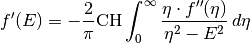
It is just a wrapper for Pythonreflectivity.KramersKroning() from Martins Zwieblers Pythonreflectivity package.

Parameters:

• energy – an ordered list/array of L energies (in eV). The energies do not have to be envenly spaced, but they should be ordered.
• f_imag – a list/array of real numbers and length L with absorption data